How to derive gradients in backprop without knowing matrix calculus (Part 1)

I believe lots of people had a hard time deriving the gradients in back propagation when they are learning about neural networks (or deep learning). You understand every example in the lecture, but when it comes to the homework you will find everything vectorized, making your skills on scalar calculus nearly useless. Perhaps matrix differentiation is the biggest obstacle for a newcomer to deep learning.

When I was learning CS231n I also struggled on deriving vectorized gradients for quite a long time. Although Karpathy has offered a tutorial on matrix calculus here, it did not make things easier because understanding the tutorial itself is also challenging. However, after struggling for weeks, I come to realize that deriving the gradients in backprop is not hard at all, as long as you are aware of the following two rules.

Rule one: Use dimension analysis.

The first rule of deriving gradients in a neural network is: do not compute matrix-matrix gradients directly unless you are very confident in your matrix calculus skills. By using dimension analysis, you can work out every matrix-matrix gradient indirectly with scalar calculus in neural networks. It can save you from all the troublesome problems like analyzing the element-wise gradients, wondering whether to sum or not, deciding the matrix multiplication order, considering when to transpose a matrix, and so on. It is also mentioned a bit in the course notes in CS231n.

So what is dimension analysis? Let’s see an example. Suppose the forward pass is $score=XW+b$, where the shape of X is NxD, W is DxC and b is 1xC, so the shape of score is NxC. Now the gradient of Loss (marked as L below) to score is given to us by the previous layer. Let’s derive the gradients of Loss to W and b.

We know that $\frac{dL}{dscore}$ is a matrix of NxC, because Loss is a scalar, so every single element’s change in score will cause Loss to change. So we have

$$\frac{dL}{dW}=\frac{dL}{dscore}\frac{dscore}{dW}$$

OK, here comes the problem. We need $\frac{dscore}{dW}$, but both score and W are matrices. How to compute that gradient? I believe many people gave up machine learning because they found they cannot even work out such a “simple” gradient and quickly lost confidence.

Let’s work it out in another way. Do not calculate $\frac{dscore}{dW}$ directly. Instead, let’s work it out with the help of the other two gradients. First, we consider the shape of it. We know $\frac{dL}{dW}$ is of DxC because it should be of the same size with W, and $\frac{dL}{dscore}$ is of NxC, so we soon found $\frac{dscore}{dW}$ should be of DxN, because (DxN) x (NxC) => (DxC). BTW, you can notice that the multiplication order is not right. It should be:

$$\frac{dL}{dW}=\frac{dscore}{dW}\frac{dL}{dscore}$$

When we know $\frac{dscore}{dW}$ is of DxN, it is almost done. Since $score = XW + b$，if they were scalars, the gradient of score to W would be X itself. X is of NxD, we want DxN, just transpose it:

$$\frac{dL}{dW}=X^T\frac{dL}{dscore}$$

That’s all.

Look, we did not compute the gradient element-by-element like $\frac{dscore_{11}}{dW_{11}}$. Instead, we worked out the desired gradient by using $\frac{dL}{dW}$ and $\frac{dL}{dscore}$ with our knowledge on pure scalar calculus. This is the most efficient way to figure out gradients in neural networks.

Why it always works? The key point is that Loss is always a scalar. The size of the gradient of a scalar to a matrix is always the same with the matrix itself. Therefore, you can always work out the matrix-matrix gradient by using two scalar-matrix gradients whose sizes are known. First, figure out the size of the unknown matrix-matrix gradient; Then, guess its content with scalar calculus; Finally, fit it with the desired shape and you are done.

What about $\frac{dL}{db}$? We know $\frac{dL}{dscore}$ is of NxC, $\frac{dL}{db}$ is 1xC, and $\frac{dscore}{db}$ looks like one, so you may have realized that $\frac{dscore}{db}$ is a matrix of 1xN whose elements are all ones, because (1xN) x (NxC) => (1xC). This is equivalent to summing up $dscore$ vertically, reducing it from NxC to 1xC.

It will be kind of hard to come up with the sum operation if you analyze it element-wise. The sum is introduced by “broadcasting” in Python. XW is a matrix of NxC, but b is only 1xC and they cannot be added together in theory. Actually, what we want to do here is to add b to every row in XW. So we duplicated b for N times, forcing it to become an NxC matrix, and then added it to XW. Therefore, when computing the gradients, you have to sum up the gradient for every row since b is actually involved in the calculation for N times. Recall the gradient rule: if a variable is involved in multiple calculations, you should sum up its gradient in each calculation. One illustration could make this more clear.

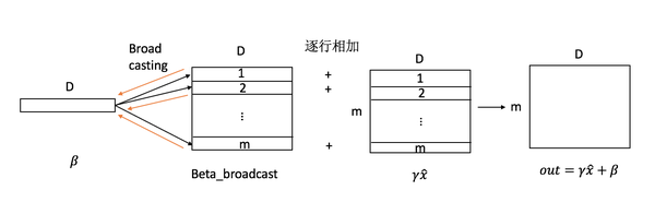
(Picture from: Zhihu)

In short, never try to compute matrix-matrix gradients directly in neural networks. Make good use of dimension analysis and it can save you tons of trouble.

Rule two will be covered in the next post.